Nowadays, we can see AI’s almost unlimited potential everywhere around us. We probably can agree on the fact that, for now, AI is successfully helping us to increase the quality of our lives. We’ll have to wait a bit longer for AI to take over the world so let’s just put this thought aside for now.

In general, applying AI for most problems we can imagine is the way to go. Usually it’s applied in cases where it’s very challenging to design a common algorithm that would solve a given issue. For example, it’s more effective to train a model to evaluate possible fraud in banking transactions rather than actually programming it.

One of the greatest challenges that AI introduces is in the medical sector, such as a patient’s diagnostics support – CT or X-ray scan recognition system and a subsequent diagnostics of the scans. But that’s just one of many possible applications for AI. It’s widely used in the fields of automotive, finance, logistics, energy, manufacturing, and the list goes on.

Tensorflow

Tensorflow, the machine learning framework from Google, quickly became popular after its release in 2015. And it has become one of the best known frameworks in the field since. Today, you can use it for quite a lot. Training models in the Python framework, applying the model in mobile apps and IOT using Tensorflow Lite, or, using Tensorflow.js, running the model in a web browser.

Convolutional neural network

We won’t go into details as we hope you already know something about neural networks and convolutional neural networks. But if this is your first time hearing about it, check out this free course that’ll give you an overview of this topic, or let us know in the comments and we’ll make sure to write an article about the basics.

In this blog post, we’ll design a simple convolutional neural network using the Tensorflow framework. We’ll describe how to freeze the model, and use it in an Android app using Tensorflow Lite. We’ll train the convolutional neural network using our own dataset that you can adjust as you like. Links for the files can be found at the end of this article. We prepared a dataset of 1,000 pictures of the duck and 1,000 pictures without it. The task of the model is to find our lost ducky.

Note: Tensorflow also has a high level API in which we don’t have to manually define matrixes for weights and biases. But we’ll create a design using a low level API in order for us to have everything under control. For comparison, you can also find a link to a complete high level implementation down below. Creating layers using a high level API is very easy:

# Convolution layer
conv1 = tf.layers.conv2d(
   inputs=input_layer,
   filters=32,
   kernel_size=[5, 5],
   padding="SAME",
   activation=tf.nn.relu)
# Pooling layer
pool1 = tf.layers.max_pooling2d(inputs=conv1, pool_size=[2, 2], strides=2)

Architecture

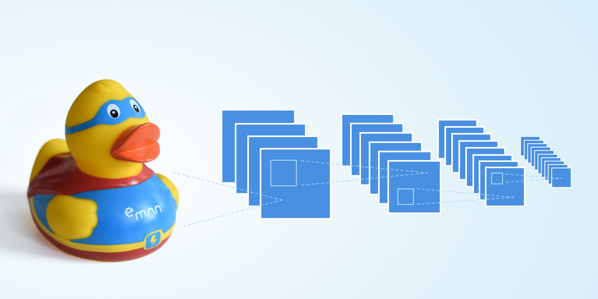
We’ll use three basic layer types for our design: convolutional, pooling and a fully connected layer. We’ll put the layers behind each other, as shown in the picture. The first part (a series of convolutional and pooling layers) is responsible for extracting a property from an image. The second part (your usual neural network) will then learn the recognition based on these properties. The added benefit of the convolutional neural network is that it already expects an image as the input, compared to a classic, fully connected neural network that works with vectors.

The input image has a 32×32 resolution and only one channel (greyscale mode). In the first part, we’ll apply 32 convolutional filters with a 5×5 size and a duty cycle of 1 to the image. For activation, we use the ReLU function throughout the duty cycle which adds non-linearity to the model. Thanks to its simplicity, ReLU does not require much computing power. Next, we add the pooling layer where the image is downsampled with a 2×2 filter and a duty cycle of 2. That’ll reduce the width and height of the image by half but the number of channels stays the same. So, from a 32x32x32 tensor we’ll get a 16x16x32 one.

input_layer = tf.placeholder(tf.float32, shape=[None, image_size * image_size], name=input_layer_name)
input_image = tf.reshape(input_layer, shape=[-1, image_size, image_size, 1])

# 1 Convolution layer
conv1_w = weight_variable([5, 5, 1, 32])
conv1_b = bias_variable([32])
conv1 = tf.nn.relu(conv2d(input_image, conv1_w) + conv1_b)
pool1 = max_pool_2x2(conv1)

We’ll add another convolutional layer with 64 5×5 filters and downsample the pooling layer once again. That’s it for extracting properties from the image and we have an 8x8x64 tensor. But before moving this tensor to the fully connected neural layer, we have to flatten it to a vector using a reshape operation.

# 2 Convolution layer
conv2_w = weight_variable([5, 5, 32, 64])
conv2_b = bias_variable([64])
conv2 = tf.nn.relu(conv2d(pool1, conv2_w) + conv2_b)
pool2 = max_pool_2x2(conv2)

# Flatten
pool2_flat = tf.reshape(pool2, [-1, 8 * 8 * 64])

Finally, we’ll add the fully connected layer with 1,024 neurons and one more output layer with two neurons, distinguishing between exactly two classes. We’ll apply softmax to the output, ensuring that the output is between <0;1> giving us sort of a probability that we either see the duck or not.

# 3 Fully connected layer
full_layer1_w = weight_variable([8 * 8 * 64, 1024])
full_layer1_b = bias_variable([1024])
full_layer1 = tf.nn.relu(tf.matmul(pool2_flat, full_layer1_w) + full_layer1_b)

# 4 Fully connected layer
full_layer2_w = weight_variable([1024, classes])
full_layer2_b = bias_variable([classes])
full_layer2 = tf.matmul(full_layer1, full_layer2_w) + full_layer2_b

# Output
output = tf.nn.softmax(full_layer2, name=output_layer_name)  # softmax output
pred = tf.argmax(output, axis=1)  # predictions

The network’s output is then the class that it “sees”. But without proper training, the results will be completely random. That’s why we add a placeholder to the graph that will be filled with the expected results during training. This variable will be used in the loss function, where we’ll express a “distance” of how far from reality the prediction is. And, while training, we’ll be minimizing this loss function using a gradient descent algorithm.

# Placeholders used for training
output_true = tf.placeholder(tf.float32, shape=[None, classes])
pred_true = tf.argmax(output_true, axis=1)

# Calculate loss function
loss = tf.reduce_mean(tf.nn.softmax_cross_entropy_with_logits_v2(labels=output_true, logits=full_layer2))
# Configure training operation
optimizer = tf.train.GradientDescentOptimizer(learning_rate).minimize(loss)

The Training

In the first part we created a graph of a model with defined operations that the model should have. During the training, we’ll be using a tensorflow session that’ll allow us to fill the graph and calculate its individual steps. The implementation is simple. First, we have a few boilerplate tensorflow lines and then we get to the training itself. This is a typical case of training with a teacher, when we present data (image) together with the expected result to the network. We are trying to create a model that’ll be as close to our function as possible. The training will use a random 32-sized batch selected from the dataset. Using this technique will allow for a more optimized usage of the descent gradient to minimize the loss function.

# Initialize variables (assign default values..)
init = tf.global_variables_initializer()
# Initialize saver
saver = tf.train.Saver()

with tf.Session() as session:
   session.run(init)
   summary_writer = tf.summary.FileWriter(train_dir, graph=tf.get_default_graph())

   for step in range(train_steps+1):
       # Get random batch
       idx = np.random.randint(train_length, size=batch_size)
       batchX = train_data[idx, :]
       batchY = train_labels[idx, :]

       # Run the optimizer
       _, train_loss, train_accuracy = session.run(
           [optimizer, loss, accuracy],
           feed_dict={input_layer: batchX,
                      output_true: batchY}
       )
       # Test training
       if step % logging_step == 0:
           test_loss, test_accuracy = session.run(
               [loss, accuracy],
               feed_dict={input_layer: eval_data,
                          output_true: eval_labels}
           )
           print("Step {0:d}: Loss = {1:.4f}, Accuracy = {2:.3f}".format(step, test_loss, test_accuracy))
       # Save checkpoint
       if step % checkpoint_step == 0:
           saver.save(session, path_current() + "/tmp/model.ckpt", global_step=step)

After launching the whole script, we should see how our model is learning and increasing the accuracy of its guesses. We save checkpoints while training the network’s parameters as these are very useful for solving complex problems if the training lasts for several hours. We can restore the session from any given checkpoint and continue the training.

Once we are satisfied with the training, we freeze the graph and export the .tflite model that we can use during production. We reload the session from the checkpoint and find the input and output in the graph because, in the production model, we only care about the path from the input to output and discard all other operations. We’ll also evaluate only individual images, not batches, so we set the tensor’s dimensions accordingly.

def freeze(checkpoint_path):
   with tf.Session() as sess:
       # First let's load meta graph and restore weights
       saver = tf.train.import_meta_graph(checkpoint_path + '.meta')
       saver.restore(sess, checkpoint_path)

       # Get the input and output tensors needed for toco
       input_tensor = sess.graph.get_tensor_by_name("input_tensor:0")
       input_tensor.set_shape([1, 1024])
       out_tensor = sess.graph.get_tensor_by_name("softmax_tensor:0")
       out_tensor.set_shape([1, 2])

       # Pass the output tensor and freeze graph
       frozen_graph_def = tf.graph_util.convert_variables_to_constants(
           sess, sess.graph_def, output_node_names=["softmax_tensor"])

   tflite_model = tf.contrib.lite.toco_convert(frozen_graph_def, [input_tensor], [out_tensor])
   open("model.tflite", "wb").write(tflite_model)
   print("Frozen model saved")

Tensorflow Lite and an Android app

Let’s create a simple Android app to see if our design works. The app will take inputs from a camera and pass them to the model for evaluation. We used the Android’s camera2 API for implementing the camera into the app. This API is a bit outside the scope of this article but if you want to know more, check out this basic example at GitHub. We add Tensorflow Lite dependency to the app’s build.gradle:

dependencies {
   implementation 'org.tensorflow:tensorflow-lite:0.1.7'
}

And we add the model into the assets, but there’s a catch. We have to set Gradle not to perform compression while building our model. So we add the following to build.gradle:

android {
   aaptOptions {
       noCompress "tflite"
   }
}

Tensorflow Lite has quite  a simple API. We create its Interpreter as follows:

val interpreter = Interpreter(loadModelFile())

Depending on the implementation, it might be necessary to pre-process the data before submitting the image to the Interpreter. We designed our network to use greyscale imaging in a 32×32 resolution, so we have to do some transformation. After the transformation, we save the image data into a field and submit it to the Interpreter:

private fun runInference(imageData: FloatArray): FloatArray {
   val input = Array(1) { _ -> imageData }
   val output = Array(1) { _ -> FloatArray(numClasses)}

   interpreter?.run(input, output)
   Log.d(TAG, "Inference run: ${Arrays.deepToString(output)}")

   return output[0]
}

And that’s all! Simple, right? The Interpreter runs the image data through the network and returns the probability output. As you probably noticed, we don’t submit only simple fields to the Interpreter so we have to create it in two dimensions, otherwise Tensorflow will complain that our dimensions don’t fit the dimensions of the tensor model. And this is the result, we found the ducky!

We mentioned the Android app only briefly… We tried to show only the important parts and catches that we encountered while using Tensorflow Lite. In any case, if you are going to implement Tensorflow Lite, make sure to check out the links below where you can find the complete source code.

Conclusion

We successfully created the convolutional neural network that recognizes a real-world object. We found all the ducks and none were harmed during our testing.

This example is mostly for fun, of course. But with a bit more work we can train the network on a different dataset or add more classes. And we can create a network that will, for example, sort products or check their quality on a production line, or something completely different like evaluating the degree of development of embryos and thus saving doctors some time. There is a plethora of uses for neural networks, one just has to look around… 🙂

Have you seen any interesting uses of neural networks? Let us know in the comments.

GitHub link to the demo model

GitHub link to the demo Android app

Sources

• The Official Tensorflow Webpage – Build a Convolutional Neural Network using Estimators
• Github – Tensorflow Lite examples (Android)
• Github – Android Camera2Basic